
Isometric Rendering in Games
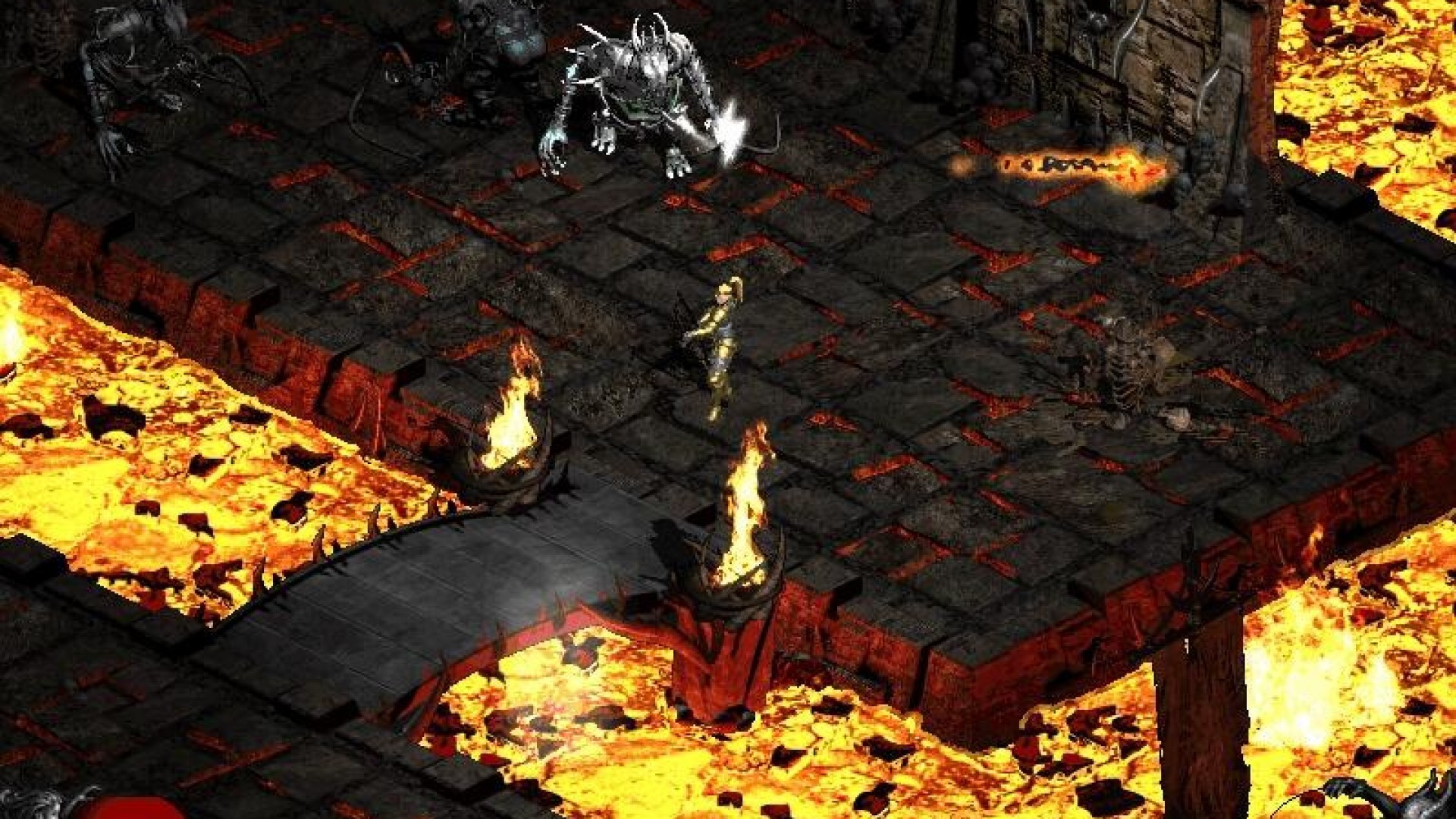
An isometric projection allows all three sides of a 3D object to be viewed on the screen. The size of the object does not depend on how far the object is from the camera or where it is located, thus allowing the object (its projection) to be rendered/authored once and re-used throughout the virtual scene. This was an immensely popular technique at a time when computers were not powerful enough to handle full-blown 3D polygon rendering: isometric rendering creates the illusion of 3D while using 2D sprites only.
This guide is an introduction to isometric rendering in games. The math is light except for maybe in the section on picking. That section is explored using different methods in the hope that at least one of them clicks with every reader. Code snippets in C for the most important topics are also presented.
Isometric Projection
An isometric projection is an axonometric projection in which all three axes are equally scaled. Let’s break that down using the following graphic from the Wikipedia:

- Orthographic: parallel projection of an object where all projection lines are orthogonal to the projection plane.
- Axonometric: single-view orthographic projection obtained by rotating an object about its axes.
- Isometric: axonometric projection that scales (foreshortens) each of the object’s axes by an equal (iso) amount. Another way to look at this is that all three axes form the same angle between them.
Isometric Coordinate System
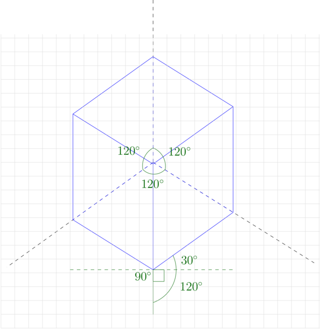
Below is a cube drawn in an isometric coordinate system. The angles between the axes are all equal, \(120^\circ\). A characteristic property of an isometric coordinate system is that the edges of the cube along the bottom form \(30^\circ\) with the horizontal axis.
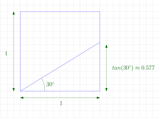
The issue with a true isometric coordinate system in isometric games is that the axes do not go exactly through the integer vertices of the grid. One way to look at this is to consider a triangle inside a square of side length 1 and forming the characteristic \(30^\circ\) angle with the x-axis. In this setup, the hypotenuse of the triangle intersects the vertical side at \(\tan(30^\circ) \approx 0.577\), a fractional number. Since a game, at the end of the day, needs to render sprites on the screen, the axes not going exactly through the integer vertices of the grid means that the game would have to sample the sprites to prevent aliasing. This was too expensive back in the day.
“Isometric” Coordinate System in Games
To work around the integer coordinates problem, isometric games use a coordinate system that establishes a 2:1 ratio, as pictured in the diagram below. Each step along the system’s \(X\) axis travels 2 pixels right and 1 pixel down. Similarly, each step along the system’s \(Y\) axis travels 2 pixels left and 1 pixel down. A sprite’s dimensions would then be an exact multiple of \(2x1\), which removes the need for antialiasing. In the cube below, for example, you can go from a vertex of the cube to another vertex of the cube by traveling 8 units to the left or right and 4 units up or down (2:1 ratio).
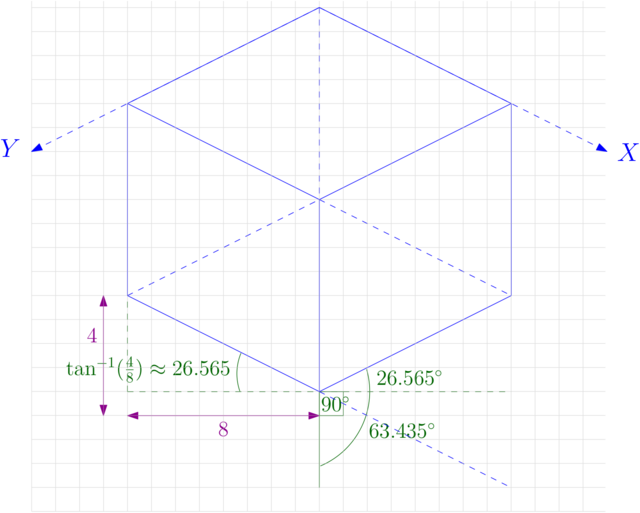
Note that the 2:1 ratio breaks the isometry and the coordinate system is no longer technically isometric. However, the game/graphics literature still calls it isometric, so we follow the same convention here. This can be seen from the fact that the characteristic angle is no longer \(30^\circ\), but \(\tan^{-1}(\frac{1}{2}) \approx 26.565^\circ\).
Also useful to note is that the axes of this “isometric” system are not orthogonal. Each forms an angle \(\approx 26.5^\circ\) with the horizontal axis, so the angle between them is \(180^\circ - 2 \cdot 26.565^\circ \approx 126.87\).
Rendering
Isometric to Cartesian
To draw a tile, we need to find the position of the tile on the screen. To do so, we need to translate the tile’s position from isometric coordinates (tile space) to Cartesian coordinates (screen space).
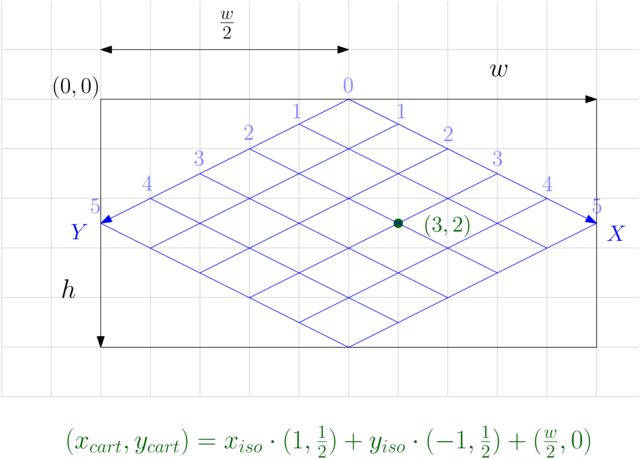
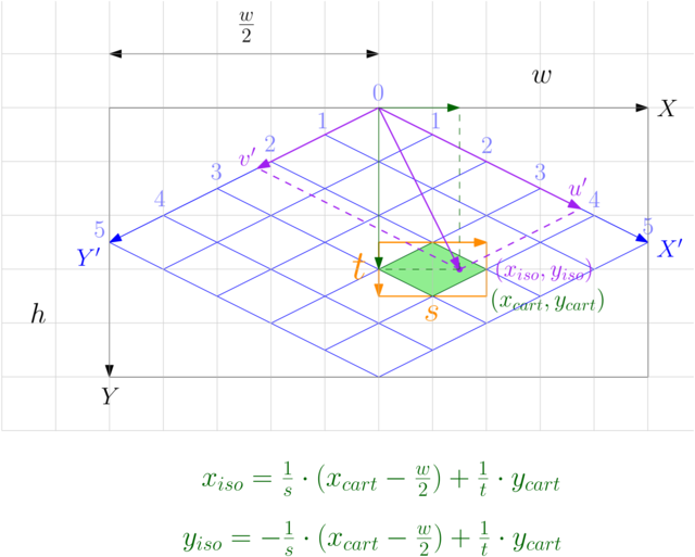
We establish the following properties for the translation. These are arbitrary and could be different, but must be used consistently throughout the following formulas:
- The isometric coordinate system’s x-axis points down and to the right.
- The isometric coordinate system’s y-axis points down and to the left.
- The origin of the isometric space is also anchored halfway through the screen for convenience, at point \((\frac{w}{2}, 0)\) in screen space.
The first two properties derive from rotating the screen-space axes clockwise. In most 2D applications, the screen space x-axis points to the right and the y-axis points down. The third property conveniently centers the isometric map on the screen.
If we assume for a second that each tile is 2x1 pixels, then we get the formula below:
Finally, generalize the tile dimensions to \(s \times t\) to get the more general formula:
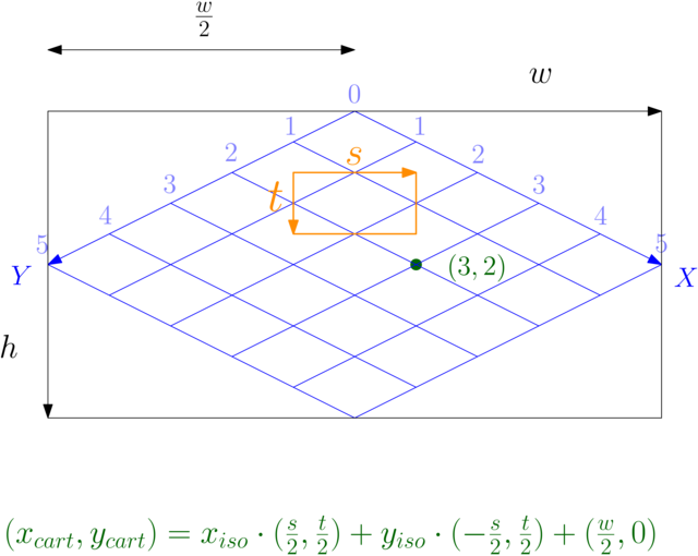
Note that as long as \(s\) and \(t\) follow a 2:1 ratio (\(s=2t\)), we can usually work out the formulas using integer math. The screen dimensions will typically be even (this can be an invariant in your engine), and then we just need to make the tile height even so that the divisions by 2 yield whole numbers.
Drawing Tiles
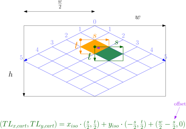
To draw a tile, we need to find out where its top-left corner lands on the screen. Then we draw the tile as you would normally draw a rectangle or a sprite.
\({TL}\) in the formula below refers to the tile’s top-left corner. It is defined using the same formula seen so far, except that we also need to offset by \(-\frac{s}{2}\), half the tile size to the left, to go from the top midpoint to the top-left corner of the tile.
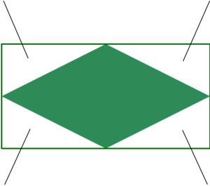
Note that for the result to look correct, we need to use tile images where the four “ears” of the image are chopped off, as shown below. This can be done with alpha masking or colour keying.
Picking
Let’s look at picking before discussing more advanced rendering topics. Picking lets us determine what tile the mouse is pointing at. At that point, you will be able to implement a basic tile editor.
Cartesian to Isometric
To determine what tile the mouse is pointing at, we need to translate the mouse coordinates from Cartesian coordinates (screen space) to isometric coordinates (tile space). This is the reverse process of the isometric-to-Cartesian formula we have seen for rendering.
To reverse the isometric-to-Cartesian formula, we will look at the following methods:
- Use basic algebraic manipulation to isolate \(x_{iso}\) and \(y_{iso}\), solving a system of 2 equations, 2 unknowns.
- Same as above, but express the original equation in terms of vector-matrix multiplication and invert a \(2x2\) matrix.
The first one is the more basic of the two. The second one is more general and succinct, but requires some familiarity with matrix algebra. Pick the method that works best for you.
Method 1: Algebraic Manipulation
Take the isometric-to-Cartesian equation and isolate \((x_{iso}, y_{iso})\):
\[\begin{align} (x_{cart}, y_{cart}) &= x_{iso} \cdot (\frac{s}{2}, \frac{t}{2}) + y_{iso} \cdot (-\frac{s}{2}, \frac{t}{2}) + (\frac{w}{2}, 0) \\\\ (x_{cart}, y_{cart}) - (\frac{w}{2}, 0) &= x_{iso} \cdot (\frac{s}{2}, \frac{t}{2}) + y_{iso} \cdot (-\frac{s}{2}, \frac{t}{2}) \\\\ (x_{cart} - \frac{w}{2}, y_{cart}) &= x_{iso} \cdot (\frac{s}{2}, \frac{t}{2}) + y_{iso} \cdot (-\frac{s}{2}, \frac{t}{2}) \end{align}\]
Above we have two unknowns and two equations, one for the x-coordinate and one for the y-coordinate. Let’s break the above equation into two:
\[\begin{align} x_{cart} - \frac{w}{2} &= \frac{s}{2}(x_{iso} - y_{iso}) \\\\ y_{cart} &= \frac{t}{2}(x_{iso} + y_{iso}) \end{align}\]
Multiply the first equation by \(t\) and the second by \(s\), then add them to eliminate \(y_{iso}\):
\[\begin{align} t \cdot (x_{cart} - \frac{w}{2}) &= \frac{ts}{2}(x_{iso} - y_{iso}) \\\\ + \; s \cdot y_{cart} &= \frac{ts}{2}(x_{iso} + y_{iso}) \\\\ \hline t \cdot (x_{cart} - \frac{w}{2}) + s \cdot y_{cart} &= ts \cdot x_{iso} \\\\ \frac{t \cdot (x_{cart} - \frac{w}{2}) + s \cdot y_{cart}}{ts} &= x_{iso} \\\\ \frac{(x_{cart} - \frac{w}{2}, y_{cart}) \cdot (t,s)}{ts} &= x_{iso} \\\\ (x_{cart} - \frac{w}{2}, y_{cart}) \cdot \frac{(t,s)}{ts} &= x_{iso} \end{align}\]
Finally, express \(y_{iso}\) in terms of \(x_{iso}\) using one of the two original equations. Let’s use the second one:
\[\begin{align} y_{cart} &= \frac{t}{2}(x_{iso} + y_{iso}) \\\\ y_{cart} &= \frac{t}{2} \cdot x_{iso} + \frac{t}{2} \cdot y_{iso} \\\\ \frac{2 (y_{cart} - \frac{t}{2} \cdot x_{iso})}{t} &= y_{iso} \\\\ \frac{2}{t} \cdot y_{cart} - x_{iso} &= y_{iso} \end{align}\]
To summarize:
\[\begin{align} x_{iso} &= (x_{cart} - \frac{w}{2}, y_{cart}) \cdot \frac{(t,s)}{ts} \\\\ y_{iso} &= \frac{2}{t} \cdot y_{cart} - x_{iso} \end{align}\]
Method 2: Matrix Inverse
Take the isometric-to-Cartesian equation and express it in matrix form:
\[\begin{align} (x_{cart}, y_{cart}) &= x_{iso} \cdot (\frac{s}{2}, \frac{t}{2}) + y_{iso} \cdot (-\frac{s}{2}, \frac{t}{2}) + (\frac{w}{2}, 0) \\\\ \begin{pmatrix}x_{cart} \\ y_{cart}\end{pmatrix} &= \begin{bmatrix} \frac{s}{2} & -\frac{s}{2} \\ \frac{t}{2} & \frac{t}{2} \end{bmatrix} \begin{pmatrix}x_{iso} \\ y_{iso}\end{pmatrix} + \begin{pmatrix}\frac{w}{2} \\ 0\end{pmatrix} \end{align}\]
Then, isolate \((x_{iso}, y_{iso})\):
\[\begin{align} \begin{pmatrix}x_{cart} \\ y_{cart}\end{pmatrix} &= \begin{bmatrix} \frac{s}{2} & -\frac{s}{2} \\ \frac{t}{2} & \frac{t}{2} \end{bmatrix} \begin{pmatrix}x_{iso} \\ y_{iso}\end{pmatrix} + \begin{pmatrix}\frac{w}{2} \\ 0\end{pmatrix} \\\\ \begin{pmatrix}x_{cart} - \frac{w}{2} \\ y_{cart}\end{pmatrix} &= \begin{bmatrix} \frac{s}{2} & -\frac{s}{2} \\ \frac{t}{2} & \frac{t}{2} \end{bmatrix} \begin{pmatrix}x_{iso} \\ y_{iso}\end{pmatrix} \\\\ \begin{bmatrix} \frac{s}{2} & -\frac{s}{2} \\ \frac{t}{2} & \frac{t}{2} \end{bmatrix}^{-1} \begin{pmatrix}x_{cart} - \frac{w}{2} \\ y_{cart}\end{pmatrix} &= \begin{pmatrix}x_{iso} \\ y_{iso}\end{pmatrix} \end{align}\]
What is left is to invert the matrix on the left.
The inverse of a \(2x2\) matrix is generally given by:
\[\begin{align} \begin{bmatrix} a & b \\ c & d \end{bmatrix}^{-1} &= \frac{1}{ad - bc} \begin{bmatrix} d & -b \\ -c & a \end{bmatrix} \end{align}\]
Applying that to our case, we get:
\[\begin{align} \begin{bmatrix} \frac{s}{2} & -\frac{s}{2} \\ \frac{t}{2} & \frac{t}{2} \end{bmatrix}^{-1} &= \frac{1}{\frac{st}{4} - \frac{-st}{4}} \begin{bmatrix} \frac{t}{2} & \frac{s}{2} \\ -\frac{t}{2} & \frac{s}{2} \end{bmatrix} \\\\ &= \frac{1}{\frac{1}{2} st} \begin{bmatrix} \frac{t}{2} & \frac{s}{2} \\ -\frac{t}{2} & \frac{s}{2} \end{bmatrix} \\\\ &= \frac{2}{st} \begin{bmatrix} \frac{t}{2} & \frac{s}{2} \\ -\frac{t}{2} & \frac{s}{2} \end{bmatrix} \\\\ &= \begin{bmatrix} \frac{2t}{2st} & \frac{2s}{2st} \\ -\frac{2t}{2st} & \frac{2s}{2st} \end{bmatrix} \\\\ &= \begin{bmatrix} \frac{1}{s} & \frac{1}{t} \\ -\frac{1}{s} & \frac{1}{t} \end{bmatrix} \\\\ \end{align}\]
It’s helpful to check that the inverse is correct by multiplying it by the original matrix. The result should be the identity:
\[\begin{align} \begin{bmatrix} \frac{1}{s} & \frac{1}{t} \\ -\frac{1}{s} & \frac{1}{t} \end{bmatrix} \begin{bmatrix} \frac{s}{2} & -\frac{s}{2} \\ \frac{t}{2} & \frac{t}{2} \end{bmatrix} &= \begin{bmatrix} \frac{s}{2s} + \frac{t}{2t} & -\frac{s}{2s} + \frac{t}{2t} \\ -\frac{s}{2s} + \frac{t}{2t} & \frac{s}{2s} + \frac{t}{2t} \end{bmatrix} \\\\ &= \begin{bmatrix} 1 & 0 \\ 0 & 1 \end{bmatrix} \end{align}\]
To summarize:
\[\begin{align} \begin{pmatrix}x_{iso} \\ y_{iso}\end{pmatrix} &= \begin{bmatrix} \frac{1}{s} & \frac{1}{t} \\ -\frac{1}{s} & \frac{1}{t} \end{bmatrix} \begin{pmatrix}x_{cart} - \frac{w}{2} \\ y_{cart}\end{pmatrix} \\\\ \end{align}\]
In non-matrix form:
\[\begin{align} x_{iso} &= \frac{1}{s} \cdot (x_{cart} - \frac{w}{2}) + \frac{1}{t} \cdot y_{cart} \\\\ y_{iso} &= -\frac{1}{s} \cdot (x_{cart} - \frac{w}{2}) + \frac{1}{t} \cdot y_{cart} \end{align}\]
Integer math?
The first two methods result in terms \(\frac{1}{s}\) and \(\frac{1}{t}\). They multiply \(x_{cart}\) and \(y_{cart}\), respectively, but the latter are not multiples of \(s\) and \(t\). So, unlike rendering, picking involves floating-point math.
Highlighting the Picked Tile
It is helpful to highlight the picked tile to debug your picker. A simple way to do this is to replace the original tile with a “picker” tile. A nicer approach is to blend the original tile with the tile. This can be done by averaging the colours or with a more general alpha blending.
\[{colour} = (1 - \alpha) \, {colour}_{picked} + \alpha \, {colour}_{picker}\]
Putting It All Together
At this point, we have all of the ingredients to put together a basic tile renderer and editor. Let’s explore the implementation of the main points seen so far.
First, define convenient data structures for representing 2D vectors:
typedef struct ivec2 {
  int x, y;
} ivec2;

typedef struct vec2 {
  double x, y;
} vec2;
Implementations for the isometric-to-Cartesian and Cartesian-to-isometric functions follow. Note that isometric-to-Cartesian works fine with integer math as long as we make the tile dimensions (\(s\) and \(t\)) and the screen width (\(w\)) multiples of 2.
/*
  s - tile width
  t - tile height
  w - screen width
*/

/// Convert isometric to Cartesian coordinates.
ivec2 iso2cart(ivec2 iso, int s, int t, int w) {
  return (ivec2){
      .x = (iso.x - iso.y) * (s / 2) + (w / 2),
      .y = (iso.x + iso.y) * (t / 2)};
}

/// Convert Cartesian to isometric coordinates, method 1.
vec2 cart2iso(vec2 cart, int s, int t, int w) {
  const double x    = cart.x - (double)(w / 2);
  const double xiso = (x * t + cart.y * s) / (double)(s * t);
  return (vec2){
      .x = (int)(xiso), .y = (int)((2.0 / (double)t) * cart.y - xiso)};
}

/// Convert Cartesian to isometric coordinates, method 2.
vec2 cart2iso(vec2 cart, int s, int t, int w) {
  const double one_over_s = 1. / (double)s;
  const double one_over_t = 1. / (double)t;
  const double x          = cart.x - (double)(w / 2);
  return (vec2){
      .x = (int)( one_over_s * x + one_over_t * cart.y),
      .y = (int)(-one_over_s * x + one_over_t * cart.y)};
}
More Rendering
Arbitrary Tile Dimensions
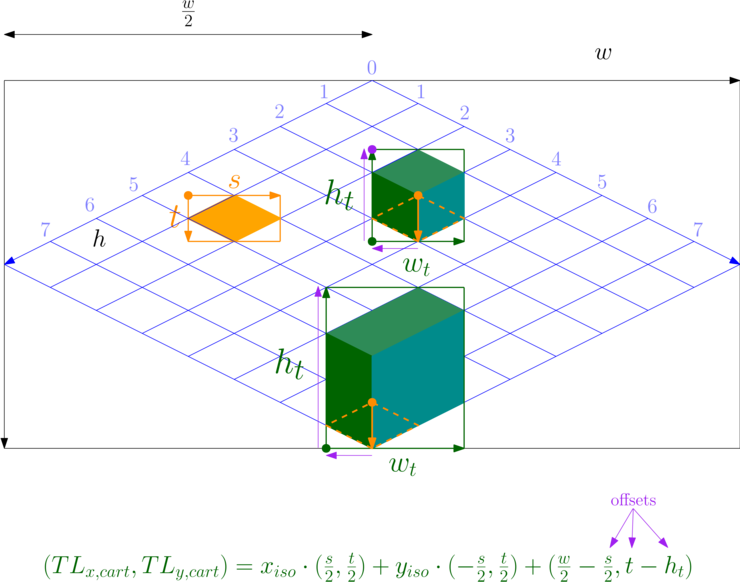
So far, the tiles we have drawn are of the same size and have no height, they are “flat” on the ground. More generally, tiles can have arbitrary widths and heights. For example, trees could span multiple tiles vertically, and tables multiple tiles horizontally. A building could span multiple tiles both vertically and horizontally.
To avoid confusion, we will refer to the tile width and height discussed so far as base tile width and base tile height (\(s\) and \(t\) in the formulas). “Tile width” and “tile height” then refer to the tile’s dimensions in pixels (different tiles may have different tile widths and heights).
To place an arbitrarily-sized tile in the world, we use the bottom-left base tile as the tile’s anchor. The tile then extends to the right and to the top of the anchor. It may also simplify an implementation to assume that the tile’s width and height are integer multiples of the base tile width and height.
To draw generally-sized tiles, we warp their origin to their bottom-left corner, which is at an offset \((-\frac{s}{2}, t)\) from the origin of the anchor (the bottom-left base-sized tile). Then, we add the tile’s height to find the tile’s top-left corner. Finally, we draw the tile as we would normally draw a sprite.
Using the top-left corner of a tile as its origin was convenient when all tiles were the same size (base tile width x base tile height), but is no longer so when the tile’s height is arbitrary.
For the rendering to be correct, we must draw the tiles back to front in screen space (top->right or top->bottom from the origin in tile space). This is so that tiles that appear closer to the camera (e.g., a building or a tree) are rendered on top of tiles that are further away (e.g., the ground). And, as usual, we must also discard the tile’s “ears”, which assume arbitrary shapes this time around.
Camera Panning
To pan the camera, we must offset the screen by the opposite amount. This affects both rendering and picking.
Rendering
Camera panning is done by adding yet another offset to the formula.
Recall the offsets seen so far:
- Drawing a point: \((\frac{w}{2}, 0)\)
- Drawing a tile of base tile dimensions \(s \times t\): \((\frac{w}{2} - \frac{s}{2}, 0)\)
- Drawing a tile of arbitrary dimensions: \((\frac{w}{2} - \frac{s}{2}, t - h_t)\)
If the camera position is given by \(\vec{c} = (c_x, c_y)\), then we offset the rendering accordingly by \(-\vec{c} = (-c_x, -c_y)\).
Picking
To pick tiles with camera panning, offset the mouse position by the camera position \(\vec{c} = (c_x, c_y)\) before plugging it into the formula:
\[(x_{cart}', \; y_{cart}') = (x_{cart} + c_x, \; y_{cart} + c_y)\]
References
Wikipedia: Axonometric projection
Wikipedia: Isometric projection